Cluster Sampling:
Intro and One-Stage

PUBHBIO 7225 Lecture 11

Generative AI acknowledgment: Google Gemini was used to generate alt text for some images

Outline

Topics

• One-stage Cluster Sampling
  • Estimation
  • Sampling weights
  • CIs
• Quantifying the Impact of Clustering
  • ICC
  • DEFF

Activities

• 11.1 One-stage Cluster Sampling

Assignments

• Problem Set 3 due Thursday 10/2/25 11:59pm via Carmen

Cluster Sampling: A Classic Example

• Want to estimate something about children in a school

• Three possible ways to sample:

  1. Take an SRS of children (from a list of all children enrolled at the school)

  2. Stratify by classroom: take an SRS of children within each classroom

  3. Take an SRS of classrooms and then sample either:

     • All children in that classroom (one-stage cluster sample)

     • An SRS of children in that classroom (two-stage cluster sample)

• In general, cluster sampling increases variance relative to an SRS (of the same number of observation units)

• If units within a cluster tend to be more similar than units between clusters → obtaining less information

• Not all outcomes (\(y\)s) would be impacted the same – which would be more impacted?

  • Classroom Example A: \(y\) = performance on a standardized test
  • Classroom Example B: \(y\) = handedness (left vs right)

So Why Would We Cluster Sample?

• We might have to: Constructing a sampling frame of observation units may be difficult, costly, or impossible.

  • Example: want to sample residents of a city, but only have a list of housing units

  • Example: studying birds in a region, but cannot list all the birds in a region (but perhaps could list geographic units which cover the region)

• Cost considerations: Cluster sampling is usually cheaper than SRS

  • Population may be widely distributed geographically

  • Population may occur in natural clusters (households, schools, etc.)

  • For the same cost you often can sample more observation units in the cluster sample compared to an SRS, thus potentially overcoming the decrease in precision caused by clustering

• Example: Target population = all incarcerated juveniles in the U.S.

  • Might be able to get a list of all incarcerated juveniles (frame), but taking an SRS would mean potentially going to a lot of locations across the U.S. (1,277 juvenile correctional facilities in 2025)

  • Cheaper to take an SRS of facilities and interview incarcerated juveniles at the sampled facilities

Vocabulary of Cluster Sampling

Primary sampling units (PSUs) = clusters = sampling units

Secondary sampling units (SSUs) = elements within clusters = observation units

• Importantly – the observation unit (SSU) is not the sampling unit (PSU)

• Can have more than two stages (e.g., children within classrooms within schools within counties…)

One-stage cluster sample = Sample all SSUs within selected PSUs (e.g., all kids in a classroom)

Two-stage cluster sample = Sample some SSUs within selected PSUs (e.g., some kids in a classroom)

• Throughout this lecture we will assume that PSUs are selected via SRS and, for two-stage cluster sampling, SSUs are selected via SRS

  • We will cover another method of selecting PSUs in a later lecture

Contrasting Cluster Sampling with Stratified Sampling

Stratified Sampling	Cluster Sampling
Each element of the population is in exactly one stratum	Each element of the population is in exactly one cluster
Strata do not overlap, and they cover the whole population	Clusters do not overlap, and they cover the whole population
Population of \(H\) strata; stratum \(h\) has \(N_h\) elements, \(N=\sum_{h=1}^H N_h\)	Population of \(N\) clusters
PSU = individual element	PSU = cluster
SSU = n/a	SSU = individual element

Contrasting Cluster Sampling with Stratified Sampling

Stratified Sampling	Cluster Sampling
SRS of elements within each stratum:	SRS of clusters and: One-stage: take all SSUs in selected PSUs 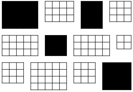Two-stage: SRS of SSUs in selected PSUs
Sample from every stratum	Only sample from some clusters

Contrasting Cluster Sampling with Stratified Sampling

Stratified Sampling	Cluster Sampling
Variance of estimate of \(\bar{y}_U\) depends on variability of \(y\) values within strata	Variance of estimate of \(\bar{y}_U\) depends primarily on variability between cluster means
Variance minimized when elements are similar within strata but stratum means differ	Variance minimized when elements are heterogeneous within cluster and cluster means are similar
Remember: homogeneous within heterogeneous between	Remember: heterogeneous within homogeneous between
Ignoring stratification often results in variance estimates that are too big	Ignoring clustering often results in variance estimates that are too small

Notation for Cluster Sampling

• \(U\) = the finite population of PSUs
• \(N\) = number of PSUs (clusters) in the population (NOT number of observation units/SSUs)
• \(M_0\) = number of SSUs in the population
• \(M_i\) = number of SSUs in PSU \(i\), with \(\displaystyle \sum_{i=1}^N M_i = M_0\)
• \(\mathcal{S}\) = a particular sample of PSUs chosen from the population
• \(\mathcal{S}_i\) = the sample of SSUs selected in PSU \(i\)
• \(n\) = number of PSUs in the sample
• \(m_i\) = number of SSUs in the sample from PSU \(i\)
  • For one-stage cluster sampling, \(m_i = M_i\) (take all SSUs in the PSU)
• \(y_{ij}\) = characteristic of interest for the \(j\)th unit in the \(i\)th PSU/cluster (not a random variable)

Activity 11.1

One-Stage Cluster Sampling (Part 1)

Example (from activity)

• Notation:

  • PSU = dorm room

  • SSU = student

  • \(N\) = Number of PSUs (rooms) = 100

  • \(M_i\) = Number of SSUs (students) in PSU (room) \(i\) = 4

  • \(M_0\) = Total number of SSUs (students) = 400

  • \(n\) = Number of PSUs (rooms) in the sample = 5

  • \(m_i\) = Number of SSUs (students) in the sample from PSU (room) \(i\) = 4 = \(M_i\) (one-stage cluster sample)

  • \(y_{ij}\) = GPA for \(j\)th SSU (student) in PSU (room) \(i\)

• You observed all students in each dorm room (all SSUs in each PSU)

  • → You observed the true total for each sampled PSU, \(\mathbf{t_i}\)

• You took an SRS of dorm rooms (PSUs)

• No new formulae! Use the results for SRS with PSU totals as the observations \((t_i)\)

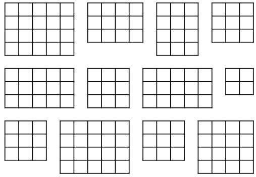
Example: A Picture

• Here’s my sample of \(n = 5\) rooms, with the \(m_i=4\) students in each room:

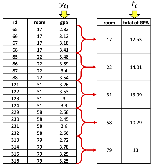
• If we collapse into one row per room, we are back to an SRS, sampling rooms and measuring the “total GPA” in each room!

One-Stage Cluster Sampling = SRS of TOTALS

• We now have an SRS of PSUs, with measured variable = total \(\mathbf{y_{ij}}\) in each room

• Can use standard SRS formulae – just substituting \(t\) (total) for \(y\) (outcome):

Quantity	Truth	Estimate
Mean (of \(t\)):	\(\displaystyle \bar{t}_U = \frac{1}{N} \sum_{i=1}^{N} t_i\)	\(\displaystyle \bar{t}= \frac{1}{n} \sum_{i\in \mathcal{S}} t_i\)
Variance:	\(\displaystyle V(t_i)=S_t^2 = \frac{1}{N-1} \sum_{i = 1}^N (t_i - \bar{t}_U)^2\)	\(\displaystyle \widehat{V}(t_i)= s_t^2=\frac{1}{n-1} \sum_{i \in\mathcal{S}_i} (t_i - \bar{t})^2\)

• And remembering that \(\bar{t}\) from our sample is a random variable, we have that:

Expected Value	Variance	Variance Estimate
\(E(\bar{t})= \bar{t}_U\)	\(\displaystyle V(\bar{t})= \left(1-\frac{n}{N}\right)\frac{S_t^2}{n}\)	\(\displaystyle \widehat{V}(\bar{t})= \left(1-\frac{n}{N}\right)\frac{s_t^2}{n}\)

• Remember, \(N\) = number of PSUs in population, \(n\) = number of PSUs in the sample

• NOT the number of SSUs!

Example (from activity)

• My SRS of dorm rooms was:

Room #	Total GPA
17	12.53
22	14.01
31	13.09
58	10.29
79	13

• \(N=100\) (number of rooms in population)

• \(n=5\) (number of rooms in sample)

\[\bar{t} = \frac{1}{n} \sum_{i\in \mathcal{S}} t_i = \frac{1}{5} (12.53 + 14.01 + 13.09 + 10.29 + 13) = \frac{62.92}{5} = 12.584\] \[\widehat{V}(t_i) = s_t^2 =\frac{1}{n-1} \sum_{i \in\mathcal{S}_i} (t_i - \bar{t})^2= \frac{1}{5-1}\left[(12.53-12.584)^2 + \cdots + (13-12.584)^2 \right]= 1.93198\]

\[\widehat{V}(\bar{t}) = \left(1-\frac{n}{N}\right)\frac{s_t^2}{n}= \left(1 - \frac{5}{100} \right) \frac{1.93198}{5} = 0.3670762\]

From TOTAL to MEAN

• We don’t really want to know about total GPA, we want to know about mean GPA

• Fortunately, we can go from totals to means fairly easily:

  • Truth: \(\bar{y}_U=\frac{\text{total of $y$}}{\text{\# of SSUs}}= \frac{t_U}{M_0}\)   →   Estimate: \(\hat{\bar{y}}_{clus}= \frac{\hat{t}_{clus}}{M_0}\)

• We have \(\bar{t}\), how can we get \(\hat{t}_{clus}\)?

  • (# of PSUs) \(\times\) (average total in a PSU) = total across all PSUs

  • Truth: \(N \times \bar{t}_U = t_U\)   →   Estimate: \(N \times \bar{t}= \hat{t}_{clus}\)

• Thus this gives us, for the mean of \(y\):

  • Truth: \(\bar{y}_U= \frac{t_U}{M_0} = \frac{N \bar{t}_U}{M_0}\)   →   Estimate: \(\hat{\bar{y}}_{clus}= \frac{\hat{t}_{clus}}{M_0} = \frac{N \bar{t}}{M_0}\)

• And of course we need variances… but conveniently \(N\) and \(M_0\) are constants!

  • Truth: \(V(\hat{\bar{y}}_{clus}) = V\left(\frac{N \bar{t}}{M_0}\right) = \frac{N^2}{M_0^2}V(\bar{t}) = \frac{N^2}{M_0^2} \left(1-\frac{n}{N}\right)\frac{S_t^2}{n}\)

One-Stage Cluster Sampling – Estimator for the Mean

Quantity	Truth	Estimate
Overall mean (of \(y\)):	\(\displaystyle \bar{y}_U = \frac{t_U}{M_0}\)	\(\displaystyle \hat{\bar{y}}_{clus}= \frac{\hat{t}_{clus}}{M_0}= \frac{N\bar{t}}{M_0}\)
Variance of \(\hat{\bar{y}}_{clus}\):	\(\displaystyle V(\hat{\bar{y}}_{clus}) = \frac{N^2}{M_0^2} \left(1-\frac{n}{N}\right)\frac{S_t^2}{n}\)	\(\displaystyle \widehat{V}(\hat{\bar{y}}_{clus}) = \frac{N^2}{M_0^2} \left(1-\frac{n}{N}\right)\frac{s_t^2}{n}\)

• Importantly, \(\hat{\bar{y}}_{clus}\) is unbiased: \(E(\hat{\bar{y}}_{clus}) =\)

• Remember,

  • \(N\) = Number of PSUs in population

  • \(n\) = Number of PSUs in sample

  • \(M_0\) = Total number of SSUs in population

• So to estimate the mean of \(y\) we…

  • calculate the average cluster total across the sampled PSUs \((\bar{t})\),

  • multiply this average by the number of PSUs \((N)\) to get a grand total \((\hat{t}_{clus})\)

  • and divide by the total number of SSUs \((M_0)\) to get an overall mean \((\hat{\bar{y}}_{clus})\)

Example (from activity)

• In my SRS of dorm rooms, I had:

  • \(N=100\) (number of rooms in population)

  • \(n=5\) (number of rooms in sample)

  • \(M_0 = 400\) (number of students in population)

  • Estimated mean PSU (room) total: \(\bar{t}= 12.584\)

  • Estimated variance of PSU (room) totals: \(s_t^2 = 1.93198\)

• My resulting estimates:

  • \(\hat{\bar{y}}_{clus}= \frac{N\bar{t}}{M_0} = \frac{100 \times 12.584}{400} = 3.146\)

  • \(\widehat{V}(\hat{\bar{y}}_{clus}) = \frac{N^2}{M_0^2} \left(1-\frac{n}{N}\right)\frac{s_t^2}{n}= \frac{100^2}{400^2} \left(1 - \frac{5}{100} \right) \frac{1.93198}{5} = 0.0229\)

  • \(\widehat{SE}(\hat{\bar{y}}_{clus}) = \sqrt{Var} = \sqrt{0.0229} = 0.151\)

Note: The true population mean GPA is \(\bar{y}_U = 2.836075\)

Sampling Weights in One-Stage Cluster Samples

• SRS of \(n\) out of \(N\) PSU   →   each PSU has probability \(n/N\) of being selected

• When clusters are sampled with equal probability (i.e., via an SRS), an SSU is included in the sample if the PSU is included in the sample

• Thus the sample weight for sampled SSU \(j\) in PSU \(i\) is: \[w_{ij} = \frac{1}{P(\text{SSU $j$ of PSU $i$ included in sample})} = \frac{1}{\pi_{ij}} = \frac{N}{n}\]

• Compare to an SRS:

  • If all PSUs had \(M_i=M\) elements, population size = \(NM\) and one-stage cluster sample has \(nM\) units

  • An SRS of \(nM\) units out of \(NM\) units: \(w_i = \frac{NM}{nM} = \frac{N}{n}\) = same as the one-stage cluster sample

  • So point estimates would be the same – but variance estimates would be different

• For the GPA cluster sample, \(w_{ij} = \frac{N}{n} = \frac{\text{\# of PSUs in \textbf{population}}}{\text{\# of PSUs in \textbf{sample}}} = \frac{100}{5} = 20\)

Confidence Intervals for One-Stage Cluster Samples

• An approximately \(\alpha\)-level confidence interval for the true mean \(\bar{y}_U\) is given by: \[\left(\hat{\bar{y}}_{clus}- t_{\alpha/2,n-1} \sqrt{\widehat{V}(\hat{\bar{y}}_{clus})}, \quad \bar{y}_{str}+ t_{\alpha/2,n-1} \sqrt{\widehat{V}(\hat{\bar{y}}_{clus})}\right)\] where \(t_{\alpha/2,n-1}\) is the \((1-\alpha/2)\)th percentile of a \(t\) distribution with DF = \(n-1\)

• Often the number of PSUs sampled is not large, thus we most often use \(t\) (instead of \(Z\))

• Again, you may see the DF “rule” written as DF = # of PSUs \(\mathbf{-}\) # of Strata

  • PSU = Primary Sampling Unit = cluster

  • If no stratification, then DF = \(n-1\) = # PSUs \(-1\)

Activity 11.1

One-Stage Cluster Sampling (Part 2)

Partitioning Variability Between and Within Clusters

• When we take a cluster sample, we often lose precision (i.e., have increased variance) (relative to SRS)

• E.g., in the activity: students living in same room have more “similar” GPAs

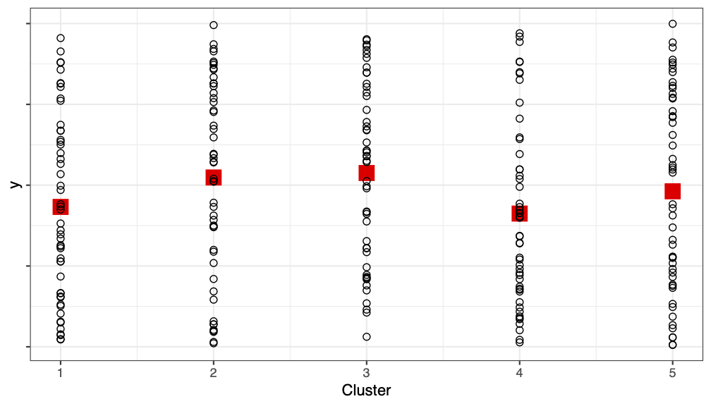
Ideally:

• We want each cluster to be a mini version of the population – like if each cluster were an SRS of the population

• If true, \(SSB \approx 0\)
  (cluster means are similar, and all the variability is within a cluster)

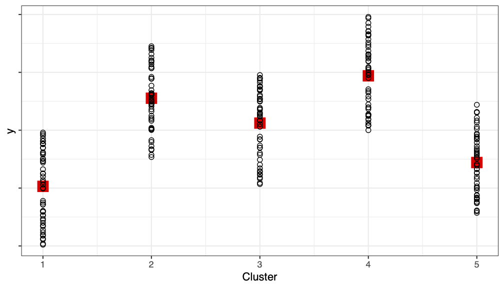
However, the reality usually is:

• Usually units are more similar within a cluster (e.g., similarity within household, similarity within dorm room)

• If true, \(SSB > 0\)

Partitioning Variability Between and Within Clusters

• We can return once again (like we did with stratification) to the idea of partitioning sums of squares to see the impact of clustering

• This is like a one-way ANOVA, where the “grouping” variable is the cluster/PSU:

\[\begin{aligned} \text{Total Sum of Squares} &{}= \text{Between PSUs} + \text{Within PSU}\\ SST &{}= SSB + SSW \\ \sum_{i=1}^N \sum_{j=1}^{M_i} (y_{ij}- \bar{y}_U)^2 &{} = \underbrace{\sum_{i=1}^N \sum_{j=1}^{M_i} (\bar{y}_{Ui} - \bar{y}_U)^2}_{\text{\textbf{between} clusters: } SSB} + \underbrace{\sum_{i=1}^N \sum_{j=1}^{M_i} (y_{ij}- \bar{y}_{Ui})^2}_{\text{\textbf{within} clusters: } SSW} \end{aligned}\]

• Between-cluster variability = how far are PSU means from overall mean (want small)

• Within-cluster variability = how far are SSUs from their PSU average (want large) (relatively speaking)

Here we are looking at the population – so, all the \(y_{ij}\), not just the sampled ones

Partitioning Variability Between and Within Clusters

When all clusters are the same size, i.e., \(M_i=m_i=M\):

ANOVA Table

Source	DF	Sum of Squares	Mean Square
Between PSUs	\(N-1\)	\(SSB=\sum_{i=1}^N \sum_{j=1}^{M} (\bar{y}_{Ui} - \bar{y}_U)^2\)	\(MSB = \frac{SSB}{N-1}\)
Within PSUs	\(NM-N\)	\(SSW=\sum_{i=1}^N \sum_{j=1}^{M} (y_{ij} - \bar{y}_{Ui})^2\)	\(MSW = \frac{SSW}{NM-N}\)
Total	\(NM-1\)	\(SST=\sum_{i=1}^N \sum_{j=1}^{M} (y_{ij} - \bar{y}_U)^2\)	\(S^2 = \frac{SST}{NM-1}\)

• Between-cluster variability: \(SSB\) = how far are PSU means \((\bar{y}_{Ui})\) from overall mean \((\bar{y}_U)\)

• Within-cluster variability: \(SSW\) = how far are SSUs \((y_{ij})\) from their PSU average \((\bar{y}_{Ui})\)

• Total variability: \(SST\) = how far are SSUs \((y_{ij})\) from overall mean \((\bar{y}_U)\)

• We will use this ANOVA decomposition to obtain a DEFF (design effect)

Intracluster Correlation Coefficient (ICC)

• Goal: quantify the impact of the clustering (how “similar” are SSUs in same PSU?)

• Assume all clusters are the same size, i.e., \(M_i = m_i = M\)

ICC = Intracluster Correlation Coefficient:   \(ICC = 1 - \frac{M}{M-1} \frac{SSW}{SST}\)

• Properties of ICC:

  • Measures how similar SSUs in the same PSU are, relative to overall variability of SSUs

  • Since \(0 \le SSW/SST \le 1\), the ICC is bounded: \(-\frac{1}{M-1} \le ICC \le 1\)

  • If all elements in a cluster are the same, then \(SSW=0\) and ICC = 1

  • If ICC \(>\) 0, cluster sampling is less efficient than simple random sampling of elements

  • The ICC is equivalent to the Pearson correlation between all pairs of observation units from the same PSU in the population

• Warning: ICC is only defined for one-stage cluster samples with equal cluster sizes

Example Calculation of ICC (from activity)

• Using the full population data, I ran a one-way ANOVA for the GPA data (\(M=\) 4 students per room, \(N=\) 100 rooms):

pop <- read.csv("./datasets/gpa.csv")
anova_model <- aov(gpa ~ factor(room), data=pop)
summary(anova_model)

              Df Sum Sq Mean Sq F value Pr(>F)    
factor(room)  99  54.37  0.5492   3.553 <2e-16 ***
Residuals    300  46.38  0.1546                   
---
Signif. codes:  0 '***' 0.001 '**' 0.01 '*' 0.05 '.' 0.1 ' ' 1

• From this we can calculate the true (theoretical) ICC:

  • \(ICC = 1 - \frac{M}{M-1} \frac{SSW}{SST} = 1 - \frac{4}{4-1} \frac{46.38}{46.38+54.37} = 0.386\)

  • \(ICC = 0.386 > 0\) so clustering will increase variance relative to SRS

Design Effect

• Just like with stratification, we use the design effect (DEFF) to quantify the impact of clustering

• Assuming all clusters are the same size (\(M_i=M\)), a one-stage cluster sample of \(n\) PSUs has \(nM\) SSUs

• Compare the variance of the mean to an SRS of size \(nM\) (out of \(NM\) SSUs)

• Design effect (DEFF) for the estimated overall mean from 1-stage cluster sample¹: \[\begin{aligned} \text{deff}(\hat{\bar{y}}_{clus}) &{}= \frac{V_{clus}(\hat{\bar{y}}_{clus})}{V_{srs}(\bar{y})} \\ &=\frac{NM-1}{NM-M}[1+(M-1)ICC] \\ & \approx 1+(M-1)ICC \quad \text{[if $N$ is large so }NM-1 \approx NM-M] \end{aligned}\]

• Thus, for each 1 SSU in an SRS, you need \([1+(M-1)ICC]\) SSUs from a one-stage cluster sample to get the same amount of information

1. Full derivation on Carmen if you’re interested (OPTIONAL)

Example Calculation of DEFF (from Activity)

• For the students (SSUs) within rooms (PSUs) the true, theoretical ICC = \(0.386\)

• \(M = 4\) students per room (SSUs per PSUs)

• DEFF = \(1+(M-1)ICC =\)

• Would need to sample more than twice as many students with clustered design as if we took an SRS (of the same number of SSUs)

• Note #1: This is the true ICC and true (theoretical) DEFF. When calculating ICC and DEFF from a cluster sample, you’ll only get estimates of these quantities.

• Note #2: In practice, clusters are rarely the same size – but we can still calculate the DEFF (using software)

Activity 11.1

One-Stage Cluster Sampling (Part 3)